You might have heard about linear regression and machine learning before. Basically linear regression is a simple statistics problem.  But what are the different types of linear regression and how to implement these in R?

Introduction to Linear Regression

Linear regression is an algorithm developed in the field of statistics. As the name suggests, linear regression assumes a linear relationship between the input variable(s) and a single output variable. The output variable, what you’re predicting, has to be continuous. The output variable can be calculated as a linear combination of the input variable(s).

There are two types of linear regression:

• Simple linear regression – only one input variable
• Multiple linear regression – multiple input variables

We will implement both today – simple linear regression from scratch and multiple linear regression with built-in R functions.

You can use a linear regression model to learn which features are important by examining coefficients. If a coefficient is close to zero, the corresponding feature is considered to be less important than if the coefficient was a large positive or negative value. 

That’s how the linear regression model generates the output. Coefficients are multiplied with corresponding input variables, and in the end, the bias (intercept) term is added.

There’s still one thing we should cover before diving into the code – assumptions of a linear regression model:

• Linear assumption — model assumes that the relationship between variables is linear
• No noise — model assumes that the input and output variables are not noisy — so remove outliers if possible
• No collinearity — model will overfit when you have highly correlated input variables
• Normal distribution — the model will make more reliable predictions if your input and output variables are normally distributed. If that’s not the case, try using some transforms on your variables to make them more normal-looking
• Rescaled inputs — use scalers or normalizer to make more reliable predictions

You should be aware of these assumptions every time you’re creating linear models. We’ll ignore most of them for the purpose of this article, as the goal is to show you the general syntax you can copy-paste between the projects. 

Simple Linear Regression from Scratch

If you have a single input variable, you’re dealing with simple linear regression. It won’t be the case most of the time, but it can’t hurt to know. A simple linear regression can be expressed as:As you can see, there are two terms you need to calculate beforehand: beta0 and beta1. You’ll first see how to calculate Beta1, as Beta0 depends on it. This is the formula:And this is the formula for Beta0:

These x’s and y’s with the bar over them represent the mean (average) of the corresponding variables.

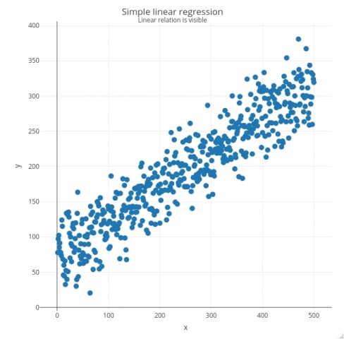
Let’s see how all of this works in action. The code snippet below generates X with 500 linearly spaced numbers between 1 and 500, and generates Y as a value from the normal distribution centered just above the corresponding X value with a bit of noise added. Both X and Y are then combined into a single data frame and visualized as a scatter plot with the plotly package:

library(plotly)
# Generate synthetic data with a linear relationship
x <- seq(from = 1, to = 500)
y <- rnorm(n = 500, mean = 0.5*x + 70, sd = 30)
lr_data <- data.frame(x, y)

# create the plot
plot_ly(data = lr_data, x = ~x, y = ~y,
marker = list(size = 10)) %>%
layout(title = list(text = paste0('Simple linear regression', '<br><sup>', 'Linear relation is visible', '</sup>'))) %>%
config(displayModeBar = F)

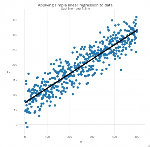
The predictions can then be obtained by applying the lr_predict() function to the vector X – they should all be on a single straight line. Finally, input data and predictions are visualized:

# Calculate coefficients
b1 <- (sum((x - mean(x)) * (y - mean(y)))) / (sum((x - mean(x))^2))
b0 <- mean(y) - b1 * mean(x)

# Define function for generating predictions
lr_predict <- function(x) { return(b0 + b1 * x) }

# Calculated predictions: Apply lr_predict() to input
lr_data$ypred <- sapply(x, lr_predict)

# Visualize input data and the best fit line
plot_ly(data = lr_data, x = ~x) %>%
add_markers(y = ~y, marker = list(size = 10)) %>%
add_lines(x = ~x, y = lr_data$ypred, line = list(color = "black", width = 5)) %>%
layout(title = list(text = paste0('Applying simple linear regression to data', '<br><sup>', 'Black line = best fit line', '</sup>')),
showlegend = FALSE) %>%
config(displayModeBar = F)

And that’s how you can implement simple linear regression in R! 

Multiple Linear Regression

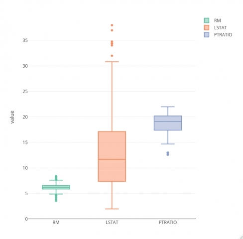
You’ll use the Boston Housing dataset to build your model. To start, the goal is to load in the dataset and check if some of the assumptions hold. Normal distribution and outlier assumptions can be checked with boxplots.

The code snippet below loads in the dataset and visualizes box plots for every feature (not the target):

library(reshape)

df <- read.csv("https://raw.githubusercontent.com/
                ginberg/boston_housing/master/housing.csv")

# Remove target variable
temp_df <- subset(df, select = -c(MEDV))
melt_df <- melt(temp_df)

plot_ly(melt_df, 
        y = ~value, 
        color = ~variable, 
        type = "box") %>%
   config(displayModeBar = F)

A degree of skew seems to be present in all input variables, and they all contain a couple of outliers. We’ll keep this blog to machine learning based, so we won’t do any data preparation/cleaning.

The next step once you’re done with preparation is to split the data into testing and training data. The caTools package is the perfect candidate for this task. 

You can train the model on the training set after the split. R has the lm function built-in, and it is used to train linear models. Inside the lm function, you’ll need to write the target variable on the left and input features on the right, separated by the  ~ sign. If you put a dot instead of feature names, it means you want to train the model on all features.

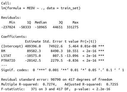
After the model is trained, you can call the summary() function to see how well it performed on the training set. Here’s a code snippet for everything discussed above:

library(caTools)
set.seed(21)

# Train/Test split, 80:20 ratio
sample_split <- sample.split(Y = df$MEDV, SplitRatio = 0.8)
train_set    <- subset(x = df, sample_split == TRUE)
test_set     <- subset(x = df, sample_split == FALSE)
# Fit the model and print summary
model        <- lm(MEDV ~ ., data = train_set)
summary(model)

The most interesting result are the P-values, displayed in the Pr(>|t|) column. Those values indicate the probability of a variable not being important for prediction. It’s common to use a 5% significance threshold, so if a P-value is 0.05 or below, we can say that there’s a low chance it is not significant for the analysis.

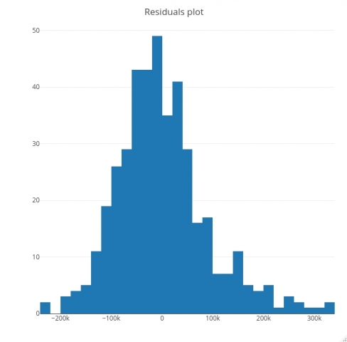
Let’s make a residuals plot now. As a general rule, if a histogram of residuals looks normally distributed, the linear model is as good as it can be. If not, it means you can improve it. Here’s the code for visualizing residuals:

# Get residuals
lm_residuals <- as.data.frame(residuals(model))

# Visualize residuals
plot_ly(x = lm_residuals

As you can see, there’s a bit of skew present due to a large error on the far right. Now, let’s make predictions on the test set. You can use the predict() function to apply the model to the test set. You can combine the actual values and predictions into a single data frame, just so the evaluation becomes easier. Here’s how:

# predict price for test_set 
predicted_prices <- predict(model, newdata = test_set) 
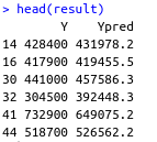
result <- data.frame(Y = test_set$MEDV, Ypred = predicted_prices)

A good way of evaluating your regression models is to look at the RMSE (Root Mean Squared Error). This metric will inform you how wrong your model is on average. In this case, it reports back the average number of price units the model is wrong:

mse  <- mean((result$Y - result$Ypred)^2)
rmse <- sqrt(mse)

In this blog you’ve learned how to train linear regression models in R. You’ve implemented a simple linear regression model entirely from scratch. After that you have implemented a multiple linear regression model with  on the real dataset. You’ve also learned how to evaluate the model through summary functions, residuals plots, and the RMSE metric. 

If you want to implement machine learning in your organization, feel free to contact me.